Download archive of sample program and outputs
The sample programs included in the book Berry Phases in Electronic Structure Theory: Electric Polarization, Orbital Magnetization and Topological Insulators (David Vanderbilt, Cambridge University Press, 2018), together with their printed and plotted outputs, can be downloaded here:
Alternatively, the sample programs and outputs can be browsed or downloaded individually below.
Note that the outputs archived here are the result of running PythTB 1.7.2 under Python 2.7, as posted in 2018 at the time of publication of the book. It is now recommended to run PythTB 1.8.0 or higher under Python 3, and newer versions of the sample programs and outputs, consistent with this environment, can be found HERE.
Table of sample programs and outputs
The links in the first column of the table will take you to the corresponding entry in the long listing below.
Listings of sample programs and outputs
Note that PDF plots are embedded as PNGs below.
1. h2o.py
#!/usr/bin/env python
from __future__ import print_function # python3 style print

# ----------------------------------------------------------
# Tight-binding model for H2O molecule
# ----------------------------------------------------------

# import the pythtb module
from pythtb import *
import numpy as np

# geometry: bond length and half bond-angle
b=1.0; angle=54.0*np.pi/180

# site energies [O(s), O(p), H(s)]
eos=-1.5; eop=-1.2; eh=-1.0

# hoppings [O(s)-H(s), O(p)-H(s)]
ts=-0.4; tp=-0.3

# define frame for defining vectors: 3D Cartesian
lat=[[1.0,0.0,0.0],[0.0,1.0,0.0],[0.0,0.0,1.0]]

# define coordinates of orbitals: O(s,px,py,pz) ; H(s) ; H(s)
orb=[ [0.,0.,0.], [0.,0.,0.], [0.,0.,0.], [0.,0.,0.],
      [b*np.cos(angle), b*np.sin(angle),0.],
      [b*np.cos(angle),-b*np.sin(angle),0.] ]

# define model
my_model=tbmodel(0,3,lat,orb)
my_model.set_onsite([eos,eop,eop,eop,eh,eh])
my_model.set_hop(ts,0,4)
my_model.set_hop(ts,0,5)
my_model.set_hop(tp*np.cos(angle),1,4)
my_model.set_hop(tp*np.cos(angle),1,5)
my_model.set_hop(tp*np.sin(angle),2,4)
my_model.set_hop(-tp*np.sin(angle),2,5)

# print model
my_model.display()

# solve model
(eval,evec)=my_model.solve_all(eig_vectors=True)

# the model is real, so OK to discard imaginary parts of eigenvectors
evec=evec.real

# optional: choose overall sign of evec according to some specified rule
# (here, we make the average oxygen p component positive)
for i in range(len(eval)):
  if sum(evec[i,1:4]) < 0:
    evec[i,:]=-evec[i,:]

# print results, setting numpy to format floats as xx.xxx
np.set_printoptions(formatter={'float': '{: 6.3f}'.format})
# print eigenvalues and real parts of eigenvectors, one to a line
print("  n   eigval   eigvec")
for n in range(6):
    print(" %2i  %7.3f  " % (n,eval[n]), evec[n,:])
Printed output
---------------------------------------
report of tight-binding model
---------------------------------------
k-space dimension           = 0
r-space dimension           = 3
number of spin components   = 1
periodic directions         = []
number of orbitals          = 6
number of electronic states = 6
lattice vectors:
 #  0  ===>  [     1.0 ,     0.0 ,     0.0 ]
 #  1  ===>  [     0.0 ,     1.0 ,     0.0 ]
 #  2  ===>  [     0.0 ,     0.0 ,     1.0 ]
positions of orbitals:
 #  0  ===>  [     0.0 ,     0.0 ,     0.0 ]
 #  1  ===>  [     0.0 ,     0.0 ,     0.0 ]
 #  2  ===>  [     0.0 ,     0.0 ,     0.0 ]
 #  3  ===>  [     0.0 ,     0.0 ,     0.0 ]
 #  4  ===>  [  0.5878 ,   0.809 ,     0.0 ]
 #  5  ===>  [  0.5878 ,  -0.809 ,     0.0 ]
site energies:
 #  0  ===>      -1.5
 #  1  ===>      -1.2
 #  2  ===>      -1.2
 #  3  ===>      -1.2
 #  4  ===>      -1.0
 #  5  ===>      -1.0
hoppings:
<  0 | H |  4 >     ===>     -0.4 +     0.0 i
<  0 | H |  5 >     ===>     -0.4 +     0.0 i
<  1 | H |  4 >     ===>  -0.1763 +     0.0 i
<  1 | H |  5 >     ===>  -0.1763 +     0.0 i
<  2 | H |  4 >     ===>  -0.2427 +     0.0 i
<  2 | H |  5 >     ===>   0.2427 +     0.0 i
hopping distances:
|  pos(  0 )  - pos(  4 ) |  =       1.0
|  pos(  0 )  - pos(  5 ) |  =       1.0
|  pos(  1 )  - pos(  4 ) |  =       1.0
|  pos(  1 )  - pos(  5 ) |  =       1.0
|  pos(  2 )  - pos(  4 ) |  =       1.0
|  pos(  2 )  - pos(  5 ) |  =       1.0

  n   eigval   eigvec
  0   -1.896   [ 0.802  0.201  0.000  0.000  0.398  0.398]
  1   -1.458   [-0.000  0.000  0.800  0.000  0.424 -0.424]
  2   -1.242   [-0.342  0.927  0.000  0.000  0.110  0.110]
  3   -1.200   [ 0.000 -0.000 -0.000  1.000 -0.000  0.000]
  4   -0.742   [-0.000  0.000  0.600  0.000 -0.566  0.566]
  5   -0.562   [ 0.490  0.317 -0.000 -0.000 -0.574 -0.574]
2. benzene.py
#!/usr/bin/env python
from __future__ import print_function # python3 style print

# ----------------------------------------------------------
# Tight-binding model for p_z states of benzene molecule
# ----------------------------------------------------------

from pythtb import *

# set up molecular geometry
lat=[[1.0,0.0],[0.0,1.0]]        # define coordinate frame: 2D Cartesian
r=1.2                            # distance of atoms from center
orb=np.zeros((6,2),dtype=float)  # initialize array for orbital positions
for i in range(6):               # define coordinates of orbitals
  angle=i*np.pi/3.0
  orb[i,:]= [r*np.cos(angle), r*np.sin(angle)]

# set site energy and hopping amplitude, respectively
ep=-0.4
t=-0.25

# define model
my_model=tbmodel(0,2,lat,orb)
my_model.set_onsite([ep,ep,ep,ep,ep,ep])
my_model.set_hop(t,0,1)
my_model.set_hop(t,1,2)
my_model.set_hop(t,2,3)
my_model.set_hop(t,3,4)
my_model.set_hop(t,4,5)
my_model.set_hop(t,5,0)

# print model
my_model.display()

# solve model and print results
(eval,evec)=my_model.solve_all(eig_vectors=True)

# print results, setting numpy to format floats as xx.xxx
np.set_printoptions(formatter={'float': '{: 6.3f}'.format})
# Print eigenvalues and real parts of eigenvectors, one to a line
print("  n   eigval   eigvec")
for n in range(6):
    print(" %2i  %7.3f  " % (n,eval[n]), evec[n,:].real)
Printed output
---------------------------------------
report of tight-binding model
---------------------------------------
k-space dimension           = 0
r-space dimension           = 2
number of spin components   = 1
periodic directions         = []
number of orbitals          = 6
number of electronic states = 6
lattice vectors:
 #  0  ===>  [     1.0 ,     0.0 ]
 #  1  ===>  [     0.0 ,     1.0 ]
positions of orbitals:
 #  0  ===>  [     1.2 ,     0.0 ]
 #  1  ===>  [     0.6 ,  1.0392 ]
 #  2  ===>  [    -0.6 ,  1.0392 ]
 #  3  ===>  [    -1.2 ,     0.0 ]
 #  4  ===>  [    -0.6 , -1.0392 ]
 #  5  ===>  [     0.6 , -1.0392 ]
site energies:
 #  0  ===>      -0.4
 #  1  ===>      -0.4
 #  2  ===>      -0.4
 #  3  ===>      -0.4
 #  4  ===>      -0.4
 #  5  ===>      -0.4
hoppings:
<  0 | H |  1 >     ===>    -0.25 +     0.0 i
<  1 | H |  2 >     ===>    -0.25 +     0.0 i
<  2 | H |  3 >     ===>    -0.25 +     0.0 i
<  3 | H |  4 >     ===>    -0.25 +     0.0 i
<  4 | H |  5 >     ===>    -0.25 +     0.0 i
<  5 | H |  0 >     ===>    -0.25 +     0.0 i
hopping distances:
|  pos(  0 )  - pos(  1 ) |  =       1.2
|  pos(  1 )  - pos(  2 ) |  =       1.2
|  pos(  2 )  - pos(  3 ) |  =       1.2
|  pos(  3 )  - pos(  4 ) |  =       1.2
|  pos(  4 )  - pos(  5 ) |  =       1.2
|  pos(  5 )  - pos(  0 ) |  =       1.2

  n   eigval   eigvec
  0   -0.900   [ 0.408  0.408  0.408  0.408  0.408  0.408]
  1   -0.650   [-0.576 -0.248  0.328  0.576  0.248 -0.328]
  2   -0.650   [-0.046 -0.521 -0.475  0.046  0.521  0.475]
  3   -0.150   [-0.349 -0.223  0.573 -0.349 -0.223  0.573]
  4   -0.150   [ 0.460 -0.532  0.073  0.460 -0.532  0.073]
  5    0.100   [ 0.408 -0.408  0.408 -0.408  0.408 -0.408]
3. li.py
#!/usr/bin/env python
from __future__ import print_function # python3 style print
# 3D model of Li on bcc lattice, with s orbitals only
from pythtb import * # import TB model class
import matplotlib.pyplot as plt
# define lattice vectors
lat=[[-0.5, 0.5, 0.5],[ 0.5,-0.5, 0.5],[ 0.5, 0.5,-0.5]]
# define coordinates of orbitals
orb=[[0.0,0.0,0.0]]
# make 3D model
my_model=tb_model(3,3,lat,orb)
# set model parameters
# lattice parameter implicitly set to a=1
Es= 4.5 # site energy
t =-1.4 # hopping parameter
# set on-site energy
my_model.set_onsite([Es])
# set hoppings along four unique bonds
# note that neighboring cell must be specified in lattice coordinates
# (the corresponding Cartesian coords are given for reference)
my_model.set_hop(t, 0, 0, [1,0,0]) # [-0.5, 0.5, 0.5] cartesian
my_model.set_hop(t, 0, 0, [0,1,0]) # [ 0.5,-0.5, 0.5] cartesian
my_model.set_hop(t, 0, 0, [0,0,1]) # [ 0.5, 0.5,-0.5] cartesian
my_model.set_hop(t, 0, 0, [1,1,1]) # [ 0.5, 0.5, 0.5] cartesian
# print tight-binding model
my_model.display()
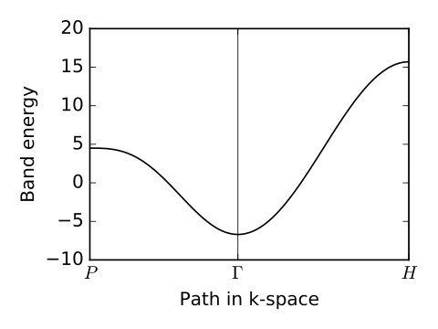
# generate k-point path and labels
# again, specified in reciprocal lattice coordinates
k_P = [0.25,0.25,0.25] # [ 0.5, 0.5, 0.5] cartesian
k_Gamma = [ 0.0, 0.0, 0.0] # [ 0.0, 0.0, 0.0] cartesian
k_H = [-0.5, 0.5, 0.5] # [ 1.0, 0.0, 0.0] cartesian
path=[k_P,k_Gamma,k_H]
label=(r'$P$',r'$\Gamma $',r'$H$')
(k_vec,k_dist,k_node)=my_model.k_path(path,101)
print('---------------------------------------')
print('starting calculation')
print('---------------------------------------')
print('Calculating bands...')
# solve for eigenenergies of hamiltonian on
# the set of k-points from above
evals=my_model.solve_all(k_vec)
# plotting of band structure
print('Plotting band structure...')
# First make a figure object
fig, ax = plt.subplots(figsize=(4.,3.))
# specify horizontal axis details
ax.set_xlim([0,k_node[-1]])
ax.set_xticks(k_node)
ax.set_xticklabels(label)
for n in range(len(k_node)):
ax.axvline(x=k_node[n], linewidth=0.5, color='k')
# plot bands
ax.plot(k_dist,evals[0],color='k')
# put title
ax.set_xlabel("Path in k-space")
ax.set_ylabel("Band energy")
# make a PDF figure of a plot
fig.tight_layout()
fig.savefig("li_bsr.pdf")
print('Done.\n')
Printed output
---------------------------------------
report of tight-binding model
---------------------------------------
k-space dimension           = 3
r-space dimension           = 3
number of spin components   = 1
periodic directions         = [0, 1, 2]
number of orbitals          = 1
number of electronic states = 1
lattice vectors:
 #  0  ===>  [    -0.5 ,     0.5 ,     0.5 ]
 #  1  ===>  [     0.5 ,    -0.5 ,     0.5 ]
 #  2  ===>  [     0.5 ,     0.5 ,    -0.5 ]
positions of orbitals:
 #  0  ===>  [     0.0 ,     0.0 ,     0.0 ]
site energies:
 #  0  ===>       4.5
hoppings:
<  0 | H |  0 + [  1 ,  0 ,  0 ] >     ===>     -1.4 +     0.0 i
<  0 | H |  0 + [  0 ,  1 ,  0 ] >     ===>     -1.4 +     0.0 i
<  0 | H |  0 + [  0 ,  0 ,  1 ] >     ===>     -1.4 +     0.0 i
<  0 | H |  0 + [  1 ,  1 ,  1 ] >     ===>     -1.4 +     0.0 i
hopping distances:
|  pos(  0 )  - pos(  0 + [  1 ,  0 ,  0 ] ) |  =     0.866
|  pos(  0 )  - pos(  0 + [  0 ,  1 ,  0 ] ) |  =     0.866
|  pos(  0 )  - pos(  0 + [  0 ,  0 ,  1 ] ) |  =     0.866
|  pos(  0 )  - pos(  0 + [  1 ,  1 ,  1 ] ) |  =     0.866

----- k_path report begin ----------
real-space lattice vectors
 [[-0.5  0.5  0.5]
 [ 0.5 -0.5  0.5]
 [ 0.5  0.5 -0.5]]
k-space metric tensor
 [[ 2.  1.  1.]
 [ 1.  2.  1.]
 [ 1.  1.  2.]]
internal coordinates of nodes
 [[ 0.25  0.25  0.25]
 [ 0.    0.    0.  ]
 [-0.5   0.5   0.5 ]]
reciprocal-space lattice vectors
 [[-0.  1.  1.]
 [ 1.  0.  1.]
 [ 1.  1.  0.]]
cartesian coordinates of nodes
 [[ 0.5  0.5  0.5]
 [ 0.   0.   0. ]
 [ 1.   0.   0. ]]
list of segments:
  length = 0.86603  from  [ 0.25  0.25  0.25]  to  [ 0.  0.  0.]
  length =     1.0  from  [ 0.  0.  0.]  to  [-0.5  0.5  0.5]
node distance list: [ 0.       0.86603  1.86603]
node index list:    [  0  46 100]
----- k_path report end ------------

---------------------------------------
starting calculation
---------------------------------------
Calculating bands...
Plotting band structure...
Done.
li_bsr.pdf
4. chain_alt.py
#!/usr/bin/env python
from __future__ import print_function # python3 style print
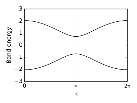
# Chain with alternating site energies and hoppings
from pythtb import *
import matplotlib.pyplot as plt
# define function to set up model for a given paramter set
def set_model(t,del_t,Delta):
# 1D model with two orbitals per cell
lat=[[1.0]]
orb=[[0.0],[0.5]]
my_model=tbmodel(1,1,lat,orb)
# alternating site energies (let average be zero)
my_model.set_onsite([Delta,-Delta])
# alternating hopping strengths
my_model.add_hop(t+del_t, 0, 1, [0])
my_model.add_hop(t-del_t, 1, 0, [1])
return my_model
# set reference hopping strength to unity to set energy scale
t=-1.0
# set alternation strengths
del_t=-0.3 # bond strength alternation
Delta= 0.4 # site energy alternation
# set up the model
my_model=set_model(t,del_t,Delta)
# construct the k-path
(k_vec,k_dist,k_node)=my_model.k_path('full',121)
k_lab=(r'0',r'$\pi$',r'$2\pi$')
# solve for eigenvalues at each point on the path
evals=my_model.solve_all(k_vec)
# set up the figure and specify details
fig, ax = plt.subplots(figsize=(4.,3.))
ax.set_xlim([0,k_node[-1]])
ax.set_xticks(k_node)
ax.set_xticklabels(k_lab)
ax.axvline(x=k_node[1],linewidth=0.5, color='k')
ax.set_xlabel("k")
ax.set_ylabel("Band energy")
# plot first and second bands
ax.plot(k_dist,evals[0],color='k')
ax.plot(k_dist,evals[1],color='k')
# save figure as a PDF
fig.tight_layout()
fig.savefig("chain_alt.pdf")
Printed output
Path in 1D BZ defined by nodes at [ 0. 0.5 1. ]
chain_alt.pdf
5. graphene.py
#!/usr/bin/env python
from __future__ import print_function # python3 style print
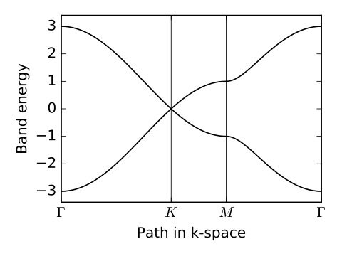
# Simple model of pi manifold of graphene
from pythtb import * # import TB model class
import matplotlib.pyplot as plt
# define lattice vectors
lat=[[1.0,0.0],[0.5,np.sqrt(3.0)/2.0]]
# define coordinates of orbitals
orb=[[1./3.,1./3.],[2./3.,2./3.]]
# make 2D tight-binding graphene model
my_model=tb_model(2,2,lat,orb)
# set model parameters
delta=0.0
t=-1.0
my_model.set_onsite([-delta,delta])
my_model.set_hop(t, 0, 1, [ 0, 0])
my_model.set_hop(t, 1, 0, [ 1, 0])
my_model.set_hop(t, 1, 0, [ 0, 1])
# print out model details
my_model.display()
# list of k-point nodes and their labels defining the path for the
# band structure plot
path=[[0.,0.],[2./3.,1./3.],[.5,.5],[0.,0.]]
label=(r'$\Gamma $',r'$K$', r'$M$', r'$\Gamma $')
# construct the k-path
nk=121
(k_vec,k_dist,k_node)=my_model.k_path(path,nk)
# solve for eigenvalues at each point on the path
evals=my_model.solve_all(k_vec)
# generate band structure plot
fig, ax = plt.subplots(figsize=(4.,3.))
# specify horizontal axis details
ax.set_xlim([0,k_node[-1]])
ax.set_ylim([-3.4,3.4])
ax.set_xticks(k_node)
ax.set_xticklabels(label)
# add vertical lines at node positions
for n in range(len(k_node)):
ax.axvline(x=k_node[n],linewidth=0.5, color='k')
# put titles
ax.set_xlabel("Path in k-space")
ax.set_ylabel("Band energy")
# plot first and second bands
ax.plot(k_dist,evals[0],color='k')
ax.plot(k_dist,evals[1],color='k')
# save figure as a PDF
fig.tight_layout()
fig.savefig("graphene.pdf")
Printed output
---------------------------------------
report of tight-binding model
---------------------------------------
k-space dimension           = 2
r-space dimension           = 2
number of spin components   = 1
periodic directions         = [0, 1]
number of orbitals          = 2
number of electronic states = 2
lattice vectors:
 #  0  ===>  [     1.0 ,     0.0 ]
 #  1  ===>  [     0.5 ,   0.866 ]
positions of orbitals:
 #  0  ===>  [  0.3333 ,  0.3333 ]
 #  1  ===>  [  0.6667 ,  0.6667 ]
site energies:
 #  0  ===>      -0.0
 #  1  ===>       0.0
hoppings:
<  0 | H |  1 + [  0 ,  0 ] >     ===>     -1.0 +     0.0 i
<  1 | H |  0 + [  1 ,  0 ] >     ===>     -1.0 +     0.0 i
<  1 | H |  0 + [  0 ,  1 ] >     ===>     -1.0 +     0.0 i
hopping distances:
|  pos(  0 )  - pos(  1 + [  0 ,  0 ] ) |  =    0.5774
|  pos(  1 )  - pos(  0 + [  1 ,  0 ] ) |  =    0.5774
|  pos(  1 )  - pos(  0 + [  0 ,  1 ] ) |  =    0.5774

----- k_path report begin ----------
real-space lattice vectors
 [[ 1.       0.     ]
 [ 0.5      0.86603]]
k-space metric tensor
 [[ 1.33333 -0.66667]
 [-0.66667  1.33333]]
internal coordinates of nodes
 [[ 0.       0.     ]
 [ 0.66667  0.33333]
 [ 0.5      0.5    ]
 [ 0.       0.     ]]
reciprocal-space lattice vectors
 [[ 1.      -0.57735]
 [ 0.       1.1547 ]]
cartesian coordinates of nodes
 [[ 0.       0.     ]
 [ 0.66667  0.     ]
 [ 0.5      0.28868]
 [ 0.       0.     ]]
list of segments:
  length = 0.66667  from  [ 0.  0.]  to  [ 0.66667  0.33333]
  length = 0.33333  from  [ 0.66667  0.33333]  to  [ 0.5  0.5]
  length = 0.57735  from  [ 0.5  0.5]  to  [ 0.  0.]
node distance list: [ 0.       0.66667  1.       1.57735]
node index list:    [  0  51  76 120]
----- k_path report end ------------
graphene.pdf
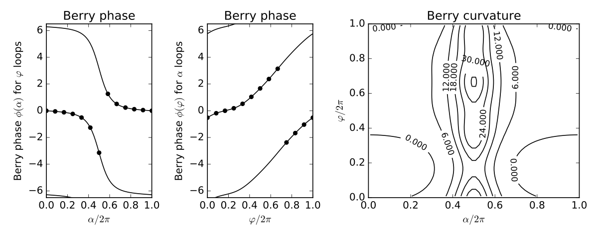
6. trimer.py
#!/usr/bin/env python
from __future__ import print_function # python3 style print

# Tight-binding model for trimer with magnetic flux

from pythtb import *
import matplotlib.pyplot as plt

# ------------------------------------------------------------
# define function to set up model for given (t0,s,phi,alpha)
# ------------------------------------------------------------
def set_model(t0,s,phi,alpha):

  # coordinate space is 2D
  lat=[[1.0,0.0],[0.0,1.0]]
  # Finite model with three orbitals forming a triangle at unit
  # distance from the origin
  sqr32=np.sqrt(3.)/2.
  orb=np.zeros((3,2),dtype=float)
  orb[0,:]=[0.,1.]          # orbital at top vertex
  orb[1,:]=[-sqr32,-0.5]    # orbital at lower left
  orb[2,:]=[ sqr32,-0.5]    # orbital at lower right

  # compute hoppings [t_01, t_12, t_20]
  # s is distortion amplitude; phi is "pseudorotation angle"
  tpio3=2.0*np.pi/3.0
  t=[ t0+s*np.cos(phi), t0+s*np.cos(phi-tpio3), t0+s*np.cos(phi-2.0*tpio3) ]

  # alpha is fraction of flux quantum passing through the triangle
  # magnetic flux correction, attached to third bond
  t[2]=t[2]*np.exp((1.j)*alpha)

  # set up model (leave site energies at zero)
  my_model=tbmodel(0,2,lat,orb)
  my_model.set_hop(t[0],0,1)
  my_model.set_hop(t[1],1,2)
  my_model.set_hop(t[2],2,0)
  return(my_model)

# ------------------------------------------------------------
# define function to return eigenvectors for given (t0,s,phi,alpha)
# ------------------------------------------------------------
def get_evecs(t0,s,phi,alpha):
  my_model=set_model(t0,s,phi,alpha)
  (eval,evec)=my_model.solve_all(eig_vectors=True)
  return(evec)        # evec[bands,orbitals]

# ------------------------------------------------------------
# begin regular execution
# ------------------------------------------------------------
# for the purposes of this problem we keep t0 and s fixed
t0 =-1.0
s  =-0.4
ref_model=set_model(t0,s,0.,1.)  # reference with phi=alpha=0
ref_model.display()

# define two pi
twopi=2.*np.pi

# ------------------------------------------------------------
# compute Berry phase for phi loop explicitly at alpha=pi/3
# ------------------------------------------------------------
alpha=np.pi/3.
n_phi=60
psi=np.zeros((n_phi,3),dtype=complex)    # initialize wavefunction array
for i in range(n_phi):
  phi=float(i)*twopi/float(n_phi)        # 60 equal intervals
  psi[i]=get_evecs(t0,s,phi,alpha)[0]    # psi[i] is short for psi[i,:]
prod=1.+0.j                              # final [0] picks out band 0
for i in range(1,n_phi):
  prod=prod*np.vdot(psi[i-1],psi[i]) # <psi_0|psi_1>...<psi_58|psi_59>
prod=prod*np.vdot(psi[-1],psi[0])    # include <psi_59|psi_0>
berry=-np.angle(prod)                # compute Berry phase
print("Explcitly computed phi Berry phase at alpha=pi/3 is %6.3f"% berry)

# ------------------------------------------------------------
# compute Berry phases for phi loops for several alpha values
# using pythtb wf_array() method
# ------------------------------------------------------------
alphas=np.linspace(0.,twopi,13)   # 0 to 2pi in 12 increments
berry_phi=np.zeros_like(alphas)      # same shape and type array (empty)
print("\nBerry phases for phi loops versus alpha")
for j,alpha in enumerate(alphas):

  # let phi range from 0 to 2pi in equally spaced steps
  n_phi=61
  phit=np.linspace(0.,twopi,n_phi)

  # set up empty wavefunction array object using pythtb wf_array()
  # creates 1D array of length [n_phi], with hidden [nbands,norbs]
  evec_array=wf_array(ref_model,[n_phi])

  # run over values of phi and fill the array
  for k,phi in enumerate(phit[0:-1]):    # skip last point of loop
    evec_array[k]=get_evecs(t0,s,phi,alpha)
  evec_array[-1]=evec_array[0]   # copy first point to last point of loop

  # now compute and store the Berry phase
  berry_phi[j]=evec_array.berry_phase([0])   # [0] specifices lowest band
  print("%3d %7.3f %7.3f"% (j, alpha, berry_phi[j]))

# ------------------------------------------------------------
# compute Berry phases for alpha loops for several phi values
# using pythtb wf_array() method
# ------------------------------------------------------------
phis=np.linspace(0.,twopi,13)   # 0 to 2pi in 12 increments
berry_alpha=np.zeros_like(phis)
print("\nBerry phases for alpha loops versus phi")
for j,phi in enumerate(phis):
  n_alpha=61
  alphat=np.linspace(0.,twopi,n_alpha)
  evec_array=wf_array(ref_model,[n_alpha])
  for k,alpha in enumerate(alphat[0:-1]):
    evec_array[k]=get_evecs(t0,s,phi,alpha)
  evec_array[-1]=evec_array[0]
  berry_alpha[j]=evec_array.berry_phase([0])
  print("%3d %7.3f %7.3f"% (j, phi, berry_alpha[j]))

# ------------------------------------------------------------
# now illustrate use of wf_array() to set up 2D array
# recompute Berry phases and compute Berry curvature
# ------------------------------------------------------------
n_phi=61
n_alp=61
n_cells=(n_phi-1)*(n_alp-1)
phi=np.linspace(0.,twopi,n_phi)
alp=np.linspace(0.,twopi,n_alp)
evec_array=wf_array(ref_model,[n_phi,n_alp])  # empty 2D wavefunction array
for i in range(n_phi):
  for j in range(n_alp):
    evec_array[i,j]=get_evecs(t0,s,phi[i],alp[j])
evec_array.impose_loop(0)   # copy first to last points in each dimension
evec_array.impose_loop(1)

bp_of_alp=evec_array.berry_phase([0],0)  # compute phi Berry phases vs. alpha
bp_of_phi=evec_array.berry_phase([0],1)  # compute alpha Berry phases vs. phi

# compute 2D array of Berry fluxes for band 0
flux=evec_array.berry_flux([0])
print("\nFlux = %7.3f = 2pi * %7.3f"% (flux, flux/twopi))
curvature=evec_array.berry_flux([0],individual_phases=True)*float(n_cells)

# ------------------------------------------------------------
# plots
# ------------------------------------------------------------
fig,ax=plt.subplots(1,3,figsize=(10,4),gridspec_kw={'width_ratios':[1,1,2]})
(ax0,ax1,ax2)=ax

ax0.set_xlim(0.,1.)
ax0.set_ylim(-6.5,6.5)
ax0.set_xlabel(r"$\alpha/2\pi$")
ax0.set_ylabel(r"Berry phase $\phi(\alpha)$ for $\varphi$ loops")
ax0.set_title("Berry phase")
for shift in (-twopi,0.,twopi):
  ax0.plot(alp/twopi,bp_of_alp+shift,color='k')
ax0.scatter(alphas/twopi,berry_phi,color='k')

ax1.set_xlim(0.,1.)
ax1.set_ylim(-6.5,6.5)
ax1.set_xlabel(r"$\varphi/2\pi$")
ax1.set_ylabel(r"Berry phase $\phi(\varphi)$ for $\alpha$ loops")
ax1.set_title("Berry phase")
for shift in (-twopi,0.,twopi):
  ax1.plot(phi/twopi,bp_of_phi+shift,color='k')
ax1.scatter(phis/twopi,berry_alpha,color='k')

X=alp[0:-1]/twopi + 0.5/float(n_alp-1)
Y=phi[0:-1]/twopi + 0.5/float(n_phi-1)
cs=ax2.contour(X,Y,curvature,colors='k')
ax2.clabel(cs, inline=1, fontsize=10)
ax2.set_title("Berry curvature")
ax2.set_xlabel(r"$\alpha/2\pi$")
ax2.set_xlim(0.,1.)
ax2.set_ylim(0.,1.)
ax2.set_ylabel(r"$\varphi/2\pi$")

fig.tight_layout()
fig.savefig("trimer.pdf")
Printed output
---------------------------------------
report of tight-binding model
---------------------------------------
k-space dimension           = 0
r-space dimension           = 2
number of spin components   = 1
periodic directions         = []
number of orbitals          = 3
number of electronic states = 3
lattice vectors:
 #  0  ===>  [     1.0 ,     0.0 ]
 #  1  ===>  [     0.0 ,     1.0 ]
positions of orbitals:
 #  0  ===>  [     0.0 ,     1.0 ]
 #  1  ===>  [  -0.866 ,    -0.5 ]
 #  2  ===>  [   0.866 ,    -0.5 ]
site energies:
 #  0  ===>       0.0
 #  1  ===>       0.0
 #  2  ===>       0.0
hoppings:
<  0 | H |  1 >     ===>     -1.4 +     0.0 i
<  1 | H |  2 >     ===>     -0.8 +     0.0 i
<  2 | H |  0 >     ===>  -0.4322 -  0.6732 i
hopping distances:
|  pos(  0 )  - pos(  1 ) |  =    1.7321
|  pos(  1 )  - pos(  2 ) |  =    1.7321
|  pos(  2 )  - pos(  0 ) |  =    1.7321

Explcitly computed phi Berry phase at alpha=pi/3 is -0.116

Berry phases for phi loops versus alpha
  0   0.000  -0.000
  1   0.524  -0.049
  2   1.047  -0.116
  3   1.571  -0.237
  4   2.094  -0.509
  5   2.618  -1.263
  6   3.142  -3.142
  7   3.665   1.263
  8   4.189   0.509
  9   4.712   0.237
 10   5.236   0.116
 11   5.760   0.049
 12   6.283   0.000

Berry phases for alpha loops versus phi
  0   0.000  -0.518
  1   0.524  -0.185
  2   1.047   0.000
  3   1.571   0.185
  4   2.094   0.518
  5   2.618   1.039
  6   3.142   1.671
  7   3.665   2.374
  8   4.189   3.142
  9   4.712  -2.374
 10   5.236  -1.671
 11   5.760  -1.039
 12   6.283  -0.518

Flux =   6.283 = 2pi *   1.000
trimer.pdf
7. chain_alt_bp.py
#!/usr/bin/env python
from __future__ import print_function # python3 style print

# Chain with alternating site energies and hoppings

from pythtb import *
import matplotlib.pyplot as plt

# define function to set up model for a given parameter set
def set_model(t,del_t,Delta):
  lat=[[1.0]]
  orb=[[0.0],[0.5]]
  my_model=tbmodel(1,1,lat,orb)
  my_model.set_onsite([Delta,-Delta])
  my_model.add_hop(t+del_t, 0, 1, [0])
  my_model.add_hop(t-del_t, 1, 0, [1])
  return my_model

# set parameters of model
t=-1.0       # average hopping
del_t=-0.3   # bond strength alternation
Delta= 0.4   # site energy alternation
my_model=set_model(t,del_t,Delta)
my_model.display()

# -----------------------------------
# explicit calculation of Berry phase
# -----------------------------------

# set up and solve the model on a discretized k mesh
nk=61          # 60 equal intervals around the unit circle
(k_vec,k_dist,k_node)=my_model.k_path('full',nk,report=False)
(eval,evec)=my_model.solve_all(k_vec,eig_vectors=True)
evec=evec[0]   # pick band=0 from evec[band,kpoint,orbital]
               # now just evec[kpoint,orbital]

# k-points 0 and 60 refer to the same point on the unit circle
# so we will work only with evec[0],...,evec[59]

# compute Berry phase of lowest band
prod=1.+0.j
for i in range(1,nk-1):            # <evec_0|evec_1>...<evec_58|evec_59>
  prod*=np.vdot(evec[i-1],evec[i]) # a*=b means a=a*b

# now compute the phase factors needed for last inner product
orb=np.array([0.0,0.5])            # relative coordinates of orbitals
phase=np.exp((-2.j)*np.pi*orb)     # construct phase factors
evec_last=phase*evec[0]            # evec[60] constructed from evec[0]
prod*=np.vdot(evec[-2],evec_last)  # include <evec_59|evec_last>

print("Berry phase is %7.3f"% (-np.angle(prod)))

# -----------------------------------
# Berry phase via the wf_array method
# -----------------------------------

evec_array=wf_array(my_model,[61])       # set array dimension
evec_array.solve_on_grid([0.])           # fill with eigensolutions
berry_phase=evec_array.berry_phase([0])  # Berry phase of bottom band

print("Berry phase is %7.3f"% berry_phase)
Printed output
---------------------------------------
report of tight-binding model
---------------------------------------
k-space dimension           = 1
r-space dimension           = 1
number of spin components   = 1
periodic directions         = [0]
number of orbitals          = 2
number of electronic states = 2
lattice vectors:
 #  0  ===>  [     1.0 ]
positions of orbitals:
 #  0  ===>  [     0.0 ]
 #  1  ===>  [     0.5 ]
site energies:
 #  0  ===>       0.4
 #  1  ===>      -0.4
hoppings:
<  0 | H |  1 + [  0 ] >     ===>     -1.3 +     0.0 i
<  1 | H |  0 + [  1 ] >     ===>     -0.7 +     0.0 i
hopping distances:
|  pos(  0 )  - pos(  1 + [  0 ] ) |  =       0.5
|  pos(  1 )  - pos(  0 + [  1 ] ) |  =       0.5

Berry phase is   2.217
Berry phase is   2.217
8. chain_3_site.py
#!/usr/bin/env python
from __future__ import print_function # python3 style print

# Chain with three sites per cell

from pythtb import *
import matplotlib.pyplot as plt

# define function to construct model
def set_model(t,delta,lmbd):
    lat=[[1.0]]
    orb=[[0.0],[1.0/3.0],[2.0/3.0]]
    model=tb_model(1,1,lat,orb)
    model.set_hop(t, 0, 1, [0])
    model.set_hop(t, 1, 2, [0])
    model.set_hop(t, 2, 0, [1])
    onsite_0=delta*(-1.0)*np.cos(2.0*np.pi*(lmbd-0.0/3.0))
    onsite_1=delta*(-1.0)*np.cos(2.0*np.pi*(lmbd-1.0/3.0))
    onsite_2=delta*(-1.0)*np.cos(2.0*np.pi*(lmbd-2.0/3.0))
    model.set_onsite([onsite_0,onsite_1,onsite_2])
    return(model)

# construct the model
t=-1.3
delta=2.0
lmbd=0.3
my_model=set_model(t,delta,lmbd)

# compute the results on a uniform k-point grid
evec_array=wf_array(my_model,[21])       # set array dimension
evec_array.solve_on_grid([0.])           # fill with eigensolutions

# obtain Berry phases and convert to Wannier center positions
#   constrained to the interval [0.,1.]
wfc0=evec_array.berry_phase([0])/(2.*np.pi)%1.
wfc1=evec_array.berry_phase([1])/(2.*np.pi)%1.
x=evec_array.berry_phase([0,1],berry_evals=True)/(2.*np.pi)%1.
gwfc0=x[0]
gwfc1=x[1]

print ("Wannier centers of bands 0 and 1:")
print(("  Individual"+" Wannier centers: "+2*"%7.4f") % (wfc0,wfc1))
print(("  Multiband "+" Wannier centers: "+2*"%7.4f") % (gwfc1,gwfc0))
print()

# construct and solve finite model by cutting 10 cells from infinite chain
finite_model=my_model.cut_piece(10,0)
(feval,fevec)=finite_model.solve_all(eig_vectors=True)

print ("Finite-chain eigenenergies associated with")
print(("Band 0:"+10*"%6.2f")% tuple(feval[0:10]))
print(("Band 1:"+10*"%6.2f")% tuple(feval[10:20]))

# find maxloc Wannier centers in each band subspace
xbar0=finite_model.position_hwf(fevec[0:10,],0)
xbar1=finite_model.position_hwf(fevec[10:20,],0)
xbarb=finite_model.position_hwf(fevec[0:20,],0)

print ("\nFinite-chain Wannier centers associated with band 0:")
print((10*"%7.4f")% tuple(xbar0))
x=10*(wfc0,)
print(("Compare with bulk:\n"+10*"%7.4f")% x)
print ("\nFinite-chain Wannier centers associated with band 1:")
print((10*"%7.4f")% tuple(xbar1))
x=10*(wfc1,)
print(("Compare with bulk:\n"+10*"%7.4f")% x)
print ("\nFirst 10 finite-chain Wannier centers associated with bands 0 and 1:")
print((10*"%7.4f")% tuple(xbarb[0:10]))
x=5*(gwfc0,gwfc1)
print(("Compare with bulk:\n"+10*"%7.4f")% x)
Printed output
Wannier centers of bands 0 and 1:
  Individual Wannier centers:  0.3188 0.9092
  Multiband  Wannier centers:  0.3419 0.8860

Finite-chain eigenenergies associated with
Band 0: -3.15 -3.12 -3.08 -3.02 -2.96 -2.88 -2.81 -2.75 -2.69 -2.66
Band 1: -0.32 -0.25 -0.14  0.01  0.17  0.34  0.51  0.66  0.77  1.16

Finite-chain Wannier centers associated with band 0:
 0.3329 1.3193 2.3188 3.3188 4.3188 5.3188 6.3188 7.3188 8.3184 9.3073
Compare with bulk:
 0.3188 0.3188 0.3188 0.3188 0.3188 0.3188 0.3188 0.3188 0.3188 0.3188

Finite-chain Wannier centers associated with band 1:
 0.0697 0.9225 1.9106 2.9093 3.9092 4.9092 5.9093 6.9100 7.9155 8.9548
Compare with bulk:
 0.9092 0.9092 0.9092 0.9092 0.9092 0.9092 0.9092 0.9092 0.9092 0.9092

First 10 finite-chain Wannier centers associated with bands 0 and 1:
 0.0195 0.3627 0.8962 1.3436 1.8871 2.3421 2.8861 3.3419 3.8860 4.3419
Compare with bulk:
 0.8860 0.3419 0.8860 0.3419 0.8860 0.3419 0.8860 0.3419 0.8860 0.3419
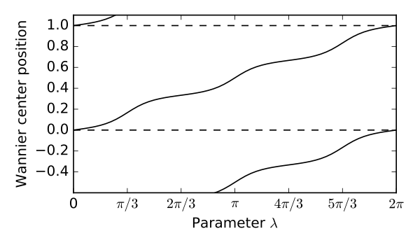
9. chain_3_cycle.py
#!/usr/bin/env python
from __future__ import print_function # python3 style print

# Chain with three sites per cell - cyclic variation

from pythtb import *
import matplotlib.pyplot as plt

# define function to construct model
def set_model(t,delta,lmbd):
    lat=[[1.0]]
    orb=[[0.0],[1.0/3.0],[2.0/3.0]]
    model=tb_model(1,1,lat,orb)
    model.set_hop(t, 0, 1, [0])
    model.set_hop(t, 1, 2, [0])
    model.set_hop(t, 2, 0, [1])
    onsite_0=delta*(-1.0)*np.cos(lmbd)
    onsite_1=delta*(-1.0)*np.cos(lmbd-2.0*np.pi/3.0)
    onsite_2=delta*(-1.0)*np.cos(lmbd-4.0*np.pi/3.0)
    model.set_onsite([onsite_0,onsite_1,onsite_2])
    return(model)

def get_xbar(band,model):
    evec_array=wf_array(model,[21])        # set array dimension
    evec_array.solve_on_grid([0.])         # fill with eigensolutions
    wfc=evec_array.berry_phase([band])/(2.*np.pi)  # Wannier centers
    return(wfc)

# set fixed parameters
t=-1.3
delta=2.0

# obtain results for an array of lambda values
lmbd=np.linspace(0.,2.*np.pi,61)
xbar=np.zeros_like(lmbd)
for j,lam in enumerate(lmbd):
    my_model=set_model(t,delta,lam)
    xbar[j]=get_xbar(0,my_model)    # Wannier center of bottom band

# enforce smooth evolution of xbar
for j in range(1,61):
    delt=xbar[j]-xbar[j-1]
    delt=-0.5+(delt+0.5)%1.  # add integer to enforce |delt| < 0.5
    xbar[j]=xbar[j-1]+delt

# set up the figure
fig, ax = plt.subplots(figsize=(5.,3.))
ax.set_xlim([0.,2.*np.pi])
ax.set_ylim([-0.6,1.1])
ax.set_xlabel(r"Parameter $\lambda$")
ax.set_ylabel(r"Wannier center position")
xlab=[r"0",r"$\pi/3$",r"$2\pi/3$",r"$\pi$",r"$4\pi/3$",r"$5\pi/3$",r"$2\pi$"]
ax.set_xticks(np.linspace(0.,2.*np.pi,num=7))
ax.set_xticklabels(xlab)
ax.plot(lmbd,xbar,'k')    # plot Wannier center and some periodic images
ax.plot(lmbd,xbar-1.,'k')
ax.plot(lmbd,xbar+1.,'k')
ax.axhline(y=1.,color='k',linestyle='dashed') # horizontal reference lines
ax.axhline(y=0.,color='k',linestyle='dashed')
fig.tight_layout()
fig.savefig("chain_3_cycle.pdf")
chain_3_cycle.pdf
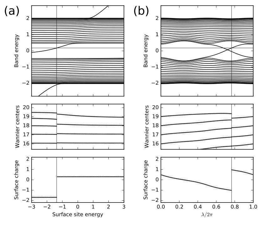
10. chain_alt_surf.py
#!/usr/bin/env python
from __future__ import print_function # python3 style print

# Chain with alternating site energies and hoppings
# Study surface properties of finite chain

from pythtb import *
import matplotlib as mpl
import matplotlib.pyplot as plt

# to set up model for given surface energy shift and lambda
def set_model(n_cell,en_shift,lmbd):

  # set parameters of model
  t=-1.0       # average hopping
  Delta=-0.4*np.cos(lmbd)   # site energy alternation
  del_t=-0.3*np.sin(lmbd)   # bond strength alternation

  # construct bulk model
  lat=[[1.0]]
  orb=[[0.0],[0.5]]
  bulk_model=tbmodel(1,1,lat,orb)
  bulk_model.set_onsite([Delta,-Delta])
  bulk_model.add_hop(t+del_t, 0, 1, [0])
  bulk_model.add_hop(t-del_t, 1, 0, [1])

  # cut chain of length n_cell and shift energy on last site
  finite_model=bulk_model.cut_piece(n_cell,0)
  finite_model.set_onsite(en_shift,ind_i=2*n_cell-1,mode='add')

  return finite_model

# set Fermi energy and number of cells
Ef=0.18
n_cell=20
n_orb=2*n_cell

# set number of parameter values to run over
n_param=101

# initialize arrays
params=np.linspace(0.,1.,n_param)
eig_sav=np.zeros((n_orb,n_param),dtype=float)
xbar_sav=np.zeros((n_orb,n_param),dtype=float)
nocc_sav=np.zeros((n_param),dtype=int)
surf_sav=np.zeros((n_param),dtype=float)
count=np.zeros((n_orb),dtype=float)

# initialize plots
mpl.rc('font',size=10)  # set global font size
fig,ax=plt.subplots(3,2,figsize=(7.,6.),
    gridspec_kw={'height_ratios':[2,1,1]},sharex="col")

# loop over two cases: vary surface site energy, or vary lambda
for mycase in ['surface energy','lambda']:

  if mycase == 'surface energy':
    (ax0,ax1,ax2)=ax[:,0]   # axes for plots in left panels
    ax0.text(-0.30,0.90,'(a)',size=22.,transform=ax0.transAxes)
    lmbd=0.15*np.pi*np.ones((n_param),dtype=float)
    en_shift=-3.0+6.0*params
    abscissa=en_shift
  elif mycase == 'lambda':
    (ax0,ax1,ax2)=ax[:,1]   # axes for plots in right panels
    ax0.text(-0.30,0.90,'(b)',size=22.,transform=ax0.transAxes)
    lmbd=params*2.*np.pi
    en_shift=0.2*np.ones((n_param),dtype=float)
    abscissa=params

  # loop over parameter values
  for j in range(n_param):

    # set up and solve model; store eigenvalues
    my_model=set_model(n_cell,en_shift[j],lmbd[j])
    (eval,evec)=my_model.solve_all(eig_vectors=True)

    # find occupied states
    nocc=(eval<Ef).sum()
    ovec=evec[0:nocc,:]

    # get Wannier centers
    xbar_sav[0:nocc,j]=my_model.position_hwf(ovec,0)

    # get electron count on each site
    # convert to charge (2 for spin; unit nuclear charge per site)
    # compute surface charge down to depth of 1/3 of chain
    for i in range(n_orb):
      count[i]=np.real(np.vdot(evec[:nocc,i],evec[:nocc,i]))
    charge=-2.*count+1.
    n_cut=int(0.67*n_orb)
    surf_sav[j]=0.5*charge[n_cut-1]+charge[n_cut:].sum()

    # save information for plots
    nocc_sav[j]=nocc
    eig_sav[:,j]=eval

  ax0.set_xlim(0.,1.)
  ax0.set_ylim(-2.8,2.8)
  ax0.set_ylabel(r"Band energy")
  ax0.axhline(y=Ef,color='k',linewidth=0.5)
  for n in range(n_orb):
    ax0.plot(abscissa,eig_sav[n,:],color='k')

  ax1.set_xlim(0.,1.)
  ax1.set_ylim(n_cell-4.6,n_cell+0.4)
  ax1.set_yticks(np.linspace(n_cell-4,n_cell,5))
  #ax1.set_ylabel(r"$\bar{x}$")
  ax1.set_ylabel(r"Wannier centers")
  for j in range(n_param):
    nocc=nocc_sav[j]
    ax1.scatter([abscissa[j]]*nocc,xbar_sav[:nocc,j],color='k',
      s=3.,marker='o',edgecolors='none')

  ax2.set_ylim(-2.2,2.2)
  ax2.set_yticks([-2.,-1.,0.,1.,2.])
  ax2.set_ylabel(r"Surface charge")
  if mycase == 'surface energy':
    ax2.set_xlabel(r"Surface site energy")
  elif mycase == 'lambda':
    ax2.set_xlabel(r"$\lambda/2\pi$")
  ax2.set_xlim(abscissa[0],abscissa[-1])
  ax2.scatter(abscissa,surf_sav,color='k',s=3.,marker='o',edgecolors='none')

  # vertical lines denote surface state at right end crossing the Fermi energy
  for j in range(1,n_param):
    if nocc_sav[j] != nocc_sav[j-1]:
      n=min(nocc_sav[j],nocc_sav[j-1])
      frac=(Ef-eig_sav[n,j-1])/(eig_sav[n,j]-eig_sav[n,j-1])
      a_jump=(1-frac)*abscissa[j-1]+frac*abscissa[j]
      if mycase == 'surface energy' or nocc_sav[j] < nocc_sav[j-1]:
        ax0.axvline(x=a_jump,color='k',linewidth=0.5)
        ax1.axvline(x=a_jump,color='k',linewidth=0.5)
        ax2.axvline(x=a_jump,color='k',linewidth=0.5)

fig.tight_layout()
plt.subplots_adjust(left=0.12,wspace=0.4)
fig.savefig("chain_alt_surf.pdf")
chain_alt_surf.pdf
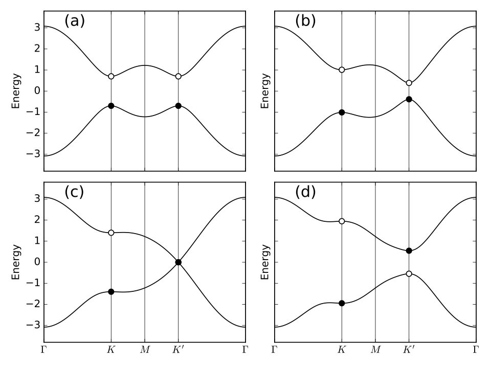
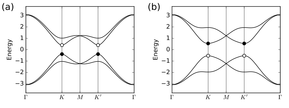
11. haldane_bsr.py
#!/usr/bin/env python
from __future__ import print_function # python3 style print

# Band structure of Haldane model

from pythtb import * # import TB model class
import matplotlib.pyplot as plt

# set model parameters
delta=0.7   # site energy shift
t=-1.0      # real first-neighbor hopping
t2=0.15     # imaginary second-neighbor hopping

def set_model(delta,t,t2):
  lat=[[1.0,0.0],[0.5,np.sqrt(3.0)/2.0]]
  orb=[[1./3.,1./3.],[2./3.,2./3.]]
  model=tb_model(2,2,lat,orb)
  model.set_onsite([-delta,delta])
  for lvec in ([ 0, 0], [-1, 0], [ 0,-1]):
    model.set_hop(t, 0, 1, lvec)
  for lvec in ([ 1, 0], [-1, 1], [ 0,-1]):
    model.set_hop(t2*1.j, 0, 0, lvec)
  for lvec in ([-1, 0], [ 1,-1], [ 0, 1]):
    model.set_hop(t2*1.j, 1, 1, lvec)
  return model

# construct path in k-space and solve model
path=[[0.,0.],[2./3.,1./3.],[.5,.5],[1./3.,2./3.], [0.,0.]]
label=(r'$\Gamma $',r'$K$', r'$M$', r'$K^\prime$', r'$\Gamma $')
(k_vec,k_dist,k_node)=set_model(delta,t,t2).k_path(path,101)

# set up band structure plots
fig, ax = plt.subplots(2,2,figsize=(8.,6.),sharex=True,sharey=True)
ax=ax.flatten()

t2_values=[0.,-0.06,-0.1347,-0.24]
labs=['(a)','(b)','(c)','(d)']
for j in range(4):

  my_model=set_model(delta,t,t2_values[j])
  evals=my_model.solve_all(k_vec)

  ax[j].set_xlim([0,k_node[-1]])
  ax[j].set_xticks(k_node)
  ax[j].set_xticklabels(label)
  for n in range(len(k_node)):
    ax[j].axvline(x=k_node[n],linewidth=0.5, color='k')
  ax[j].set_ylabel("Energy")
  ax[j].set_ylim(-3.8,3.8)
  for n in range(2):
    ax[j].plot(k_dist,evals[n],color='k')

  # filled or open dots at K and K' following band inversion
  for m in [1,3]:
    kk=k_node[m]
    (en,ev)=my_model.solve_one(path[m],eig_vectors=True)
    if np.abs(ev[0,0]) > np.abs(ev[0,1]):   #ev[band,orb]
      en=[en[1],en[0]]
    ax[j].scatter(kk,en[0],s=40.,marker='o',edgecolors='k',facecolors='w',zorder=4)
    ax[j].scatter(kk,en[1],s=40.,marker='o',color='k',zorder=6)

  ax[j].text(0.20,3.1,labs[j],size=18.)

# save figure as a PDF
fig.tight_layout()
fig.savefig("haldane_bsr.pdf")
Printed output
----- k_path report begin ----------
real-space lattice vectors
 [[ 1.       0.     ]
 [ 0.5      0.86603]]
k-space metric tensor
 [[ 1.33333 -0.66667]
 [-0.66667  1.33333]]
internal coordinates of nodes
 [[ 0.       0.     ]
 [ 0.66667  0.33333]
 [ 0.5      0.5    ]
 [ 0.33333  0.66667]
 [ 0.       0.     ]]
reciprocal-space lattice vectors
 [[ 1.      -0.57735]
 [ 0.       1.1547 ]]
cartesian coordinates of nodes
 [[ 0.       0.     ]
 [ 0.66667  0.     ]
 [ 0.5      0.28868]
 [ 0.33333  0.57735]
 [ 0.       0.     ]]
list of segments:
  length = 0.66667  from  [ 0.  0.]  to  [ 0.66667  0.33333]
  length = 0.33333  from  [ 0.66667  0.33333]  to  [ 0.5  0.5]
  length = 0.33333  from  [ 0.5  0.5]  to  [ 0.33333  0.66667]
  length = 0.66667  from  [ 0.33333  0.66667]  to  [ 0.  0.]
node distance list: [ 0.       0.66667  1.       1.33333  2.     ]
node index list:    [  0  33  50  67 100]
----- k_path report end ------------
haldane_bsr.pdf
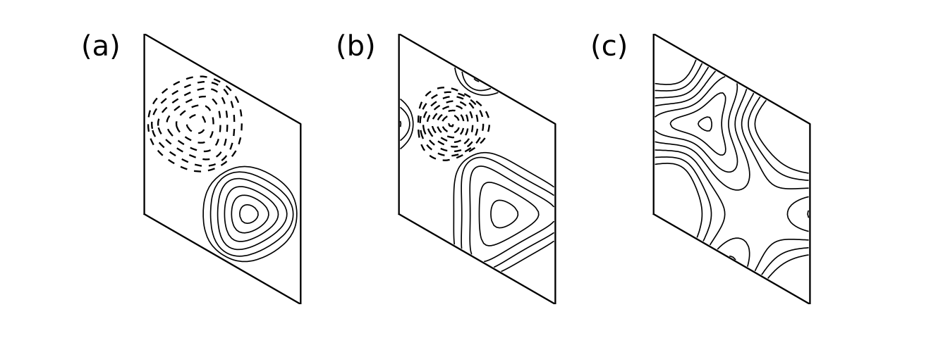
12. haldane_bcurv.py
#!/usr/bin/env python
from __future__ import print_function # python3 style print

# Berry curvature of Haldane model

from pythtb import * # import TB model class
import matplotlib.pyplot as plt

# define setup of Haldane model
def set_model(delta,t,t2):
  lat=[[1.0,0.0],[0.5,np.sqrt(3.0)/2.0]]
  orb=[[1./3.,1./3.],[2./3.,2./3.]]
  model=tb_model(2,2,lat,orb)
  model.set_onsite([-delta,delta])
  for lvec in ([ 0, 0], [-1, 0], [ 0,-1]):
    model.set_hop(t, 0, 1, lvec)
  for lvec in ([ 1, 0], [-1, 1], [ 0,-1]):
    model.set_hop(t2*1.j, 0, 0, lvec)
  for lvec in ([-1, 0], [ 1,-1], [ 0, 1]):
    model.set_hop(t2*1.j, 1, 1, lvec)
  return model

# miscellaneous setup
delta=0.7   # site energy shift
t=-1.0      # real first-neighbor hopping

nk=61
dk=2.*np.pi/(nk-1)
k0=(np.arange(nk-1)+0.5)/(nk-1)
kx=np.zeros((nk-1,nk-1),dtype=float)
ky=np.zeros((nk-1,nk-1),dtype=float)
sq3o2=np.sqrt(3.)/2.
for i in range(nk-1):
  for j in range(nk-1):
    kx[i,j]=sq3o2*k0[i]
    ky[i,j]= -0.5*k0[i]+k0[j]

fig,ax=plt.subplots(1,3,figsize=(11,4))
labs=['(a)','(b)','(c)']

# compute Berry curvature and Chern number for three values of t2
for j,t2 in enumerate([0.,-0.06,-0.24]):
  my_model=set_model(delta,t,t2)
  my_array=wf_array(my_model,[nk,nk])
  my_array.solve_on_grid([0.,0.])
  bcurv=my_array.berry_flux([0],individual_phases=True)/(dk*dk)
  chern=my_array.berry_flux([0])/(2.*np.pi)
  print('Chern number =',"%8.5f"%chern)

  # make contour plot of Berry curvature
  pos_lvls= 0.02*np.power(2.,np.linspace(0,8,9))
  neg_lvls=-0.02*np.power(2.,np.linspace(8,0,9))
  ax[j].contour(kx,ky,bcurv,levels=pos_lvls,colors='k')
  ax[j].contour(kx,ky,bcurv,levels=neg_lvls,colors='k',linewidths=1.4)

  # remove rectangular box and draw parallelogram, etc.
  ax[j].xaxis.set_visible(False)
  ax[j].yaxis.set_visible(False)
  for loc in ["top","bottom","left","right"]:
    ax[j].spines[loc].set_visible(False)
  ax[j].set(aspect=1.)
  ax[j].plot([0,sq3o2,sq3o2,0,0],[0,-0.5,0.5,1,0],color='k',linewidth=1.4)
  ax[j].set_xlim(-0.05,sq3o2+0.05)
  ax[j].text(-.35,0.88,labs[j],size=24.)

fig.savefig("haldane_bcurv.pdf")
Printed output
Chern number = -0.00000
Chern number =  0.00000
Chern number =  1.00000
haldane_bcurv.pdf
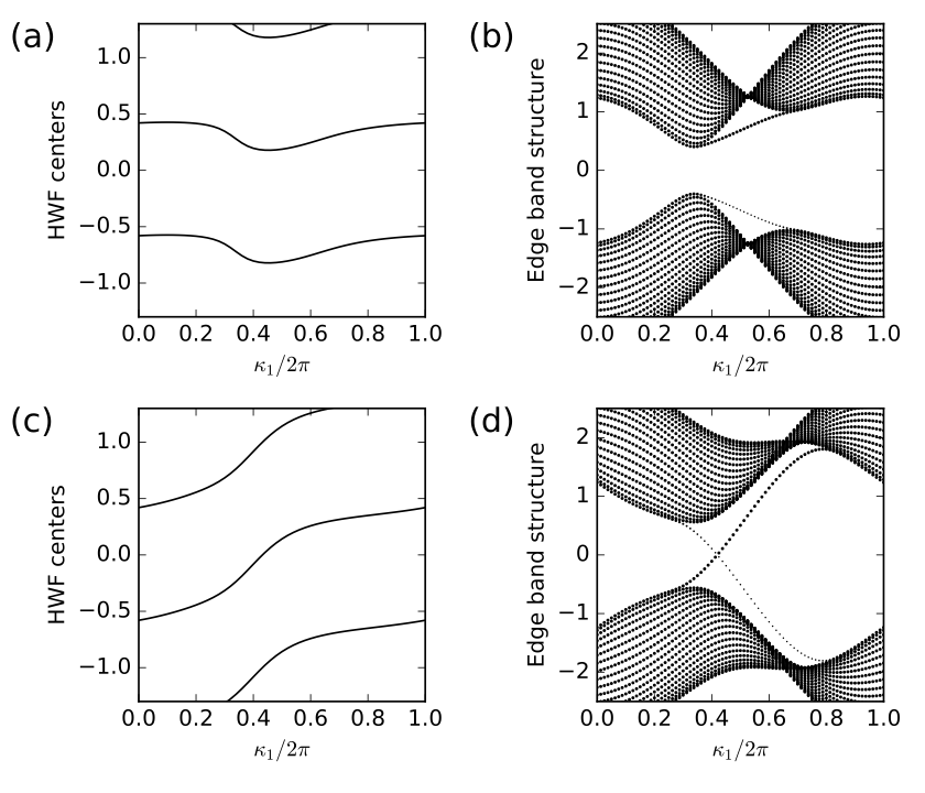
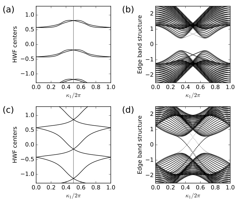
13. haldane_topo.py
#!/usr/bin/env python
from __future__ import print_function # python3 style print

# Band structure of Haldane model

from pythtb import * # import TB model class
import matplotlib.pyplot as plt

# define setup of Haldane model
def set_model(delta,t,t2):
  lat=[[1.0,0.0],[0.5,np.sqrt(3.0)/2.0]]
  orb=[[1./3.,1./3.],[2./3.,2./3.]]
  model=tb_model(2,2,lat,orb)
  model.set_onsite([-delta,delta])
  for lvec in ([ 0, 0], [-1, 0], [ 0,-1]):
    model.set_hop(t, 0, 1, lvec)
  for lvec in ([ 1, 0], [-1, 1], [ 0,-1]):
    model.set_hop(t2*1.j, 0, 0, lvec)
  for lvec in ([-1, 0], [ 1,-1], [ 0, 1]):
    model.set_hop(t2*1.j, 1, 1, lvec)
  return model

# set model parameters and construct bulk model
delta=0.7   # site energy shift
t=-1.0      # real first-neighbor hopping
nk=51

# For the purposes of plot labels:
#   Real space is (r1,r2) in reduced coordinates
#   Reciprocal space is (k1,k2) in reduced coordinates
# Below, following Python, these are (r0,r1) and (k0,k1)

# set up figures
fig,ax=plt.subplots(2,2,figsize=(7,6))

# run over two choices of t2
for j2,t2 in enumerate([-0.06,-0.24]):

  # solve bulk model on grid and get hybrid Wannier centers along r1
  # as a function of k0
  my_model=set_model(delta,t,t2)
  my_array=wf_array(my_model,[nk,nk])
  my_array.solve_on_grid([0.,0.])
  rbar_1 = my_array.berry_phase([0],1,contin=True)/(2.*np.pi)

  # set up and solve ribbon model that is finite along direction 1
  width=20
  nkr=81
  ribbon_model=my_model.cut_piece(width,fin_dir=1,glue_edgs=False)
  (k_vec,k_dist,k_node)=ribbon_model.k_path('full',nkr,report=False)
  (rib_eval,rib_evec)=ribbon_model.solve_all(k_vec,eig_vectors=True)

  nbands=rib_eval.shape[0]
  (ax0,ax1)=ax[j2,:]

  # hybrid Wannier center flow
  k0=np.linspace(0.,1.,nk)
  ax0.set_xlim(0.,1.)
  ax0.set_ylim(-1.3,1.3)
  ax0.set_xlabel(r"$\kappa_1/2\pi$")
  ax0.set_ylabel(r"HWF centers")
  for shift in (-2.,-1.,0.,1.):
    ax0.plot(k0,rbar_1+shift,color='k')

  # edge band structure
  k0=np.linspace(0.,1.,nkr)
  ax1.set_xlim(0.,1.)
  ax1.set_ylim(-2.5,2.5)
  ax1.set_xlabel(r"$\kappa_1/2\pi$")
  ax1.set_ylabel(r"Edge band structure")
  for (i,kv) in enumerate(k0):

    # find expectation value <r1> at i'th k-point along direction k0
    pos_exp=ribbon_model.position_expectation(rib_evec[:,i],dir=1)

    # assign weight in [0,1] to be 1 except for edge states near bottom
    weight=3.0*pos_exp/width
    for j in range(nbands):
      weight[j]=min(weight[j],1.)

    # scatterplot with symbol size proportional to assigned weight
    s=ax1.scatter([k_vec[i]]*nbands, rib_eval[:,i],
         s=0.6+2.5*weight, c='k', marker='o', edgecolors='none')

# save figure as a PDF
aa=ax.flatten()
for i,lab in enumerate(['(a)','(b)','(c)','(d)']):
  aa[i].text(-0.45,0.92,lab,size=18.,transform=aa[i].transAxes)
fig.tight_layout()
plt.subplots_adjust(left=0.15,wspace=0.6)
fig.savefig("haldane_topo.pdf")
haldane_topo.pdf
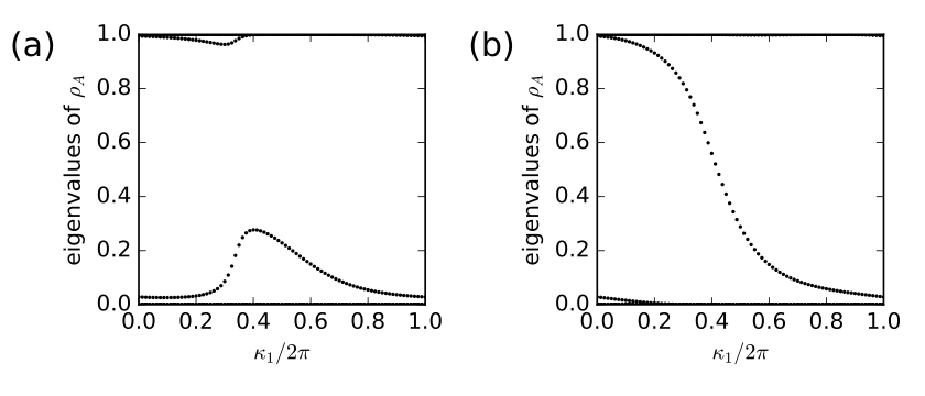
14. haldane_entang.py
#!/usr/bin/env python
from __future__ import print_function # python3 style print

# Entanglement spectrum of Haldane model

from pythtb import * # import TB model class
import matplotlib.pyplot as plt

# define setup of Haldane model
def set_model(delta,t,t2):
  lat=[[1.0,0.0],[0.5,np.sqrt(3.0)/2.0]]
  orb=[[1./3.,1./3.],[2./3.,2./3.]]
  model=tb_model(2,2,lat,orb)
  model.set_onsite([-delta,delta])
  for lvec in ([ 0, 0], [-1, 0], [ 0,-1]):
    model.set_hop(t, 0, 1, lvec)
  for lvec in ([ 1, 0], [-1, 1], [ 0,-1]):
    model.set_hop(t2*1.j, 0, 0, lvec)
  for lvec in ([-1, 0], [ 1,-1], [ 0, 1]):
    model.set_hop(t2*1.j, 1, 1, lvec)
  return model

# set model parameters and construct bulk model
delta=0.7   # site energy shift
t=-1.0      # real first-neighbor hopping

# set up figures
fig,ax=plt.subplots(1,2,figsize=(7,3))

# run over two choices of t2
for j2,t2 in enumerate([-0.10,-0.24]):

  my_model=set_model(delta,t,t2)

  # set up and solve ribbon model that is finite along direction 1
  width=20
  nkr=81
  ribbon_model=my_model.cut_piece(width,fin_dir=1,glue_edgs=False)
  (k_vec,k_dist,k_node)=ribbon_model.k_path('full',nkr,report=False)
  (rib_eval,rib_evec)=ribbon_model.solve_all(k_vec,eig_vectors=True)

  nbands=rib_eval.shape[0]
  ax1=ax[j2]

  # entanglement spectrum
  k0=np.linspace(0.,1.,nkr)
  ax1.set_xlim(0.,1.)
  ax1.set_ylim(0.,1)
  ax1.set_xlabel(r"$\kappa_1/2\pi$")
  ax1.set_ylabel(r"eigenvalues of $\rho_A$")

  (nband,nk,norb)=rib_evec.shape
  ncut=norb/2
  nocc=nband/2

  for (i,kv) in enumerate(k0):

    # construct reduced density matrix for half of the chain
    dens_mat=np.zeros((ncut,ncut),dtype=complex)
    for nb in range(nocc):
      for j1 in range(ncut):
        for j2 in range(ncut):
          dens_mat[j1,j2] += np.conj(rib_evec[nb,i,j1])*rib_evec[nb,i,j2]

    # diagonalize
    spect=np.real(np.linalg.eigvals(dens_mat))
    # scatterplot
    s=ax1.scatter([k_vec[i]]*nocc, spect,
         s=4, c='k', marker='o', edgecolors='none')

# save figure as a PDF
aa=ax.flatten()
for i,lab in enumerate(['(a)','(b)']):
  aa[i].text(-0.45,0.92,lab,size=18.,transform=aa[i].transAxes)
fig.tight_layout()
plt.subplots_adjust(left=0.15,wspace=0.6)
fig.savefig("haldane_entang.pdf")
haldane_entang.pdf
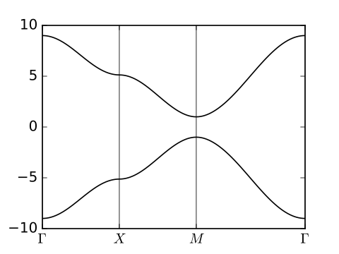
15. checkerboard.py
#!/usr/bin/env python
from __future__ import print_function # python3 style print

from pythtb import * # import TB model class
import matplotlib.pyplot as plt

# set geometry
lat=[[1.0,0.0],[0.0,1.0]]
orb=[[0.0,0.0],[0.5,0.5]]
my_model=tbmodel(2,2,lat,orb)

# set model
Delta  = 5.0
t_0    = 1.0
tprime = 0.4
my_model.set_sites([-Delta,Delta])
my_model.add_hop(-t_0, 0, 0, [ 1, 0])
my_model.add_hop(-t_0, 0, 0, [ 0, 1])
my_model.add_hop( t_0, 1, 1, [ 1, 0])
my_model.add_hop( t_0, 1, 1, [ 0, 1])
my_model.add_hop( tprime   , 1, 0, [ 1, 1])
my_model.add_hop( tprime*1j, 1, 0, [ 0, 1])
my_model.add_hop(-tprime   , 1, 0, [ 0, 0])
my_model.add_hop(-tprime*1j, 1, 0, [ 1, 0])
my_model.display()

# generate k-point path and labels and solve Hamiltonian
path=[[0.0,0.0],[0.0,0.5],[0.5,0.5],[0.0,0.0]]
k_lab=(r'$\Gamma $',r'$X$', r'$M$', r'$\Gamma $')
(k_vec,k_dist,k_node)=my_model.k_path(path,121)
evals=my_model.solve_all(k_vec)

# plot band structure
fig, ax = plt.subplots(figsize=(4.,3.))
ax.set_xlim([0,k_node[-1]])
ax.set_xticks(k_node)
ax.set_xticklabels(k_lab)
for n in range(len(k_node)):
  ax.axvline(x=k_node[n], linewidth=0.5, color='k')
ax.plot(k_dist,evals[0],color='k')
ax.plot(k_dist,evals[1],color='k')
fig.savefig("checkerboard_bsr.pdf")
Printed output
---------------------------------------
report of tight-binding model
---------------------------------------
k-space dimension           = 2
r-space dimension           = 2
number of spin components   = 1
periodic directions         = [0, 1]
number of orbitals          = 2
number of electronic states = 2
lattice vectors:
 #  0  ===>  [     1.0 ,     0.0 ]
 #  1  ===>  [     0.0 ,     1.0 ]
positions of orbitals:
 #  0  ===>  [     0.0 ,     0.0 ]
 #  1  ===>  [     0.5 ,     0.5 ]
site energies:
 #  0  ===>      -5.0
 #  1  ===>       5.0
hoppings:
<  0 | H |  0 + [  1 ,  0 ] >     ===>     -1.0 +     0.0 i
<  0 | H |  0 + [  0 ,  1 ] >     ===>     -1.0 +     0.0 i
<  1 | H |  1 + [  1 ,  0 ] >     ===>      1.0 +     0.0 i
<  1 | H |  1 + [  0 ,  1 ] >     ===>      1.0 +     0.0 i
<  1 | H |  0 + [  1 ,  1 ] >     ===>      0.4 +     0.0 i
<  1 | H |  0 + [  0 ,  1 ] >     ===>      0.0 +     0.4 i
<  1 | H |  0 + [  0 ,  0 ] >     ===>     -0.4 +     0.0 i
<  1 | H |  0 + [  1 ,  0 ] >     ===>     -0.0 -     0.4 i
hopping distances:
|  pos(  0 )  - pos(  0 + [  1 ,  0 ] ) |  =       1.0
|  pos(  0 )  - pos(  0 + [  0 ,  1 ] ) |  =       1.0
|  pos(  1 )  - pos(  1 + [  1 ,  0 ] ) |  =       1.0
|  pos(  1 )  - pos(  1 + [  0 ,  1 ] ) |  =       1.0
|  pos(  1 )  - pos(  0 + [  1 ,  1 ] ) |  =    0.7071
|  pos(  1 )  - pos(  0 + [  0 ,  1 ] ) |  =    0.7071
|  pos(  1 )  - pos(  0 + [  0 ,  0 ] ) |  =    0.7071
|  pos(  1 )  - pos(  0 + [  1 ,  0 ] ) |  =    0.7071

----- k_path report begin ----------
real-space lattice vectors
 [[ 1.  0.]
 [ 0.  1.]]
k-space metric tensor
 [[ 1.  0.]
 [ 0.  1.]]
internal coordinates of nodes
 [[ 0.   0. ]
 [ 0.   0.5]
 [ 0.5  0.5]
 [ 0.   0. ]]
reciprocal-space lattice vectors
 [[ 1.  0.]
 [ 0.  1.]]
cartesian coordinates of nodes
 [[ 0.   0. ]
 [ 0.   0.5]
 [ 0.5  0.5]
 [ 0.   0. ]]
list of segments:
  length =     0.5  from  [ 0.  0.]  to  [ 0.   0.5]
  length =     0.5  from  [ 0.   0.5]  to  [ 0.5  0.5]
  length = 0.70711  from  [ 0.5  0.5]  to  [ 0.  0.]
node distance list: [ 0.       0.5      1.       1.70711]
node index list:    [  0  35  70 120]
----- k_path report end ------------
checkerboard_bsr.pdf
16. kanemele_bsr.py
#!/usr/bin/env python
from __future__ import print_function # python3 style print

# Tight-binding 2D Kane-Mele model
# C.L. Kane and E.J. Mele, PRL 95, 146802 (2005)

from pythtb import * # import TB model class
import matplotlib.pyplot as plt

# set model parameters
delta=0.7     # site energy
t=-1.0        # spin-independent first-neighbor hop
rashba=0.05   # spin-flip first-neighbor hop
soc_list=[-0.06,-0.24] # spin-dependent second-neighbor hop

def set_model(t,soc,rashba,delta):

  # set up Kane-Mele model
  lat=[[1.0,0.0],[0.5,np.sqrt(3.0)/2.0]]
  orb=[[1./3.,1./3.],[2./3.,2./3.]]
  model=tb_model(2,2,lat,orb,nspin=2)
  model.set_onsite([delta,-delta])

  # definitions of Pauli matrices
  sigma_x=np.array([0.,1.,0.,0])
  sigma_y=np.array([0.,0.,1.,0])
  sigma_z=np.array([0.,0.,0.,1])
  r3h =np.sqrt(3.0)/2.0
  sigma_a= 0.5*sigma_x-r3h*sigma_y
  sigma_b= 0.5*sigma_x+r3h*sigma_y
  sigma_c=-1.0*sigma_x

  # spin-independent first-neighbor hops
  for lvec in ([ 0, 0], [-1, 0], [ 0,-1]):
    model.set_hop(t, 0, 1, lvec)
  # spin-dependent second-neighbor hops
  for lvec in ([ 1, 0], [-1, 1], [ 0,-1]):
    model.set_hop(soc*1.j*sigma_z, 0, 0, lvec)
  for lvec in ([-1, 0], [ 1,-1], [ 0, 1]):
    model.set_hop(soc*1.j*sigma_z, 1, 1, lvec)
  # spin-flip first-neighbor hops
  model.set_hop(1.j*rashba*sigma_a, 0, 1, [ 0, 0], mode="add")
  model.set_hop(1.j*rashba*sigma_b, 0, 1, [-1, 0], mode="add")
  model.set_hop(1.j*rashba*sigma_c, 0, 1, [ 0,-1], mode="add")

  return model

# construct path in k-space and solve model
path=[[0.,0.],[2./3.,1./3.],[.5,.5],[1./3.,2./3.], [0.,0.]]
label=(r'$\Gamma $',r'$K$', r'$M$', r'$K^\prime$', r'$\Gamma $')
(k_vec,k_dist,k_node)=set_model(t,0.,rashba,delta).k_path(path,101)

# set up band structure plots
fig, ax = plt.subplots(1,2,figsize=(8.,3.))

labs=['(a)','(b)']
for j in range(2):

  my_model=set_model(t,soc_list[j],rashba,delta)
  evals=my_model.solve_all(k_vec)

  ax[j].set_xlim([0,k_node[-1]])
  ax[j].set_xticks(k_node)
  ax[j].set_xticklabels(label)
  for n in range(len(k_node)):
    ax[j].axvline(x=k_node[n],linewidth=0.5, color='k')
  ax[j].set_ylabel("Energy")
  ax[j].set_ylim(-3.8,3.8)
  for n in range(4):
    ax[j].plot(k_dist,evals[n],color='k')

  for m in [1,3]:
    kk=k_node[m]
    en=my_model.solve_one(path[m])
    en=en[1:3]  # pick out second and third bands
    if j==1:    # exchange them in second plot
      en=[en[1],en[0]]
    ax[j].scatter(kk,en[0],s=40.,marker='o',color='k',zorder=6)
    ax[j].scatter(kk,en[1],s=40.,marker='o',edgecolors='k',facecolors='w',zorder=4)

  ax[j].text(-0.45,3.5,labs[j],size=18.)

# save figure as a PDF
fig.tight_layout()
plt.subplots_adjust(wspace=0.35)
fig.savefig("kanemele_bsr.pdf")
Printed output
----- k_path report begin ----------
real-space lattice vectors
 [[ 1.       0.     ]
 [ 0.5      0.86603]]
k-space metric tensor
 [[ 1.33333 -0.66667]
 [-0.66667  1.33333]]
internal coordinates of nodes
 [[ 0.       0.     ]
 [ 0.66667  0.33333]
 [ 0.5      0.5    ]
 [ 0.33333  0.66667]
 [ 0.       0.     ]]
reciprocal-space lattice vectors
 [[ 1.      -0.57735]
 [ 0.       1.1547 ]]
cartesian coordinates of nodes
 [[ 0.       0.     ]
 [ 0.66667  0.     ]
 [ 0.5      0.28868]
 [ 0.33333  0.57735]
 [ 0.       0.     ]]
list of segments:
  length = 0.66667  from  [ 0.  0.]  to  [ 0.66667  0.33333]
  length = 0.33333  from  [ 0.66667  0.33333]  to  [ 0.5  0.5]
  length = 0.33333  from  [ 0.5  0.5]  to  [ 0.33333  0.66667]
  length = 0.66667  from  [ 0.33333  0.66667]  to  [ 0.  0.]
node distance list: [ 0.       0.66667  1.       1.33333  2.     ]
node index list:    [  0  33  50  67 100]
----- k_path report end ------------
kanemele_bsr.pdf
17. kanemele_topo.py
#!/usr/bin/env python
from __future__ import print_function # python3 style print

# Tight-binding 2D Kane-Mele model
# C.L. Kane and E.J. Mele, PRL 95, 146802 (2005)

from pythtb import * # import TB model class
import matplotlib.pyplot as plt

# set model parameters
delta=0.7     # site energy
t=-1.0        # spin-independent first-neighbor hop
soc=0.06      # spin-dependent second-neighbor hop
rashba=0.05   # spin-flip first-neighbor hop
soc_list=[-0.06,-0.24] # spin-dependent second-neighbor hop

def set_model(t,soc,rashba,delta):

  # set up Kane-Mele model
  lat=[[1.0,0.0],[0.5,np.sqrt(3.0)/2.0]]
  orb=[[1./3.,1./3.],[2./3.,2./3.]]
  model=tb_model(2,2,lat,orb,nspin=2)
  model.set_onsite([delta,-delta])

  # definitions of Pauli matrices
  sigma_x=np.array([0.,1.,0.,0])
  sigma_y=np.array([0.,0.,1.,0])
  sigma_z=np.array([0.,0.,0.,1])
  r3h =np.sqrt(3.0)/2.0
  sigma_a= 0.5*sigma_x-r3h*sigma_y
  sigma_b= 0.5*sigma_x+r3h*sigma_y
  sigma_c=-1.0*sigma_x

  # spin-independent first-neighbor hops
  for lvec in ([ 0, 0], [-1, 0], [ 0,-1]):
    model.set_hop(t, 0, 1, lvec)
  # spin-dependent second-neighbor hops
  for lvec in ([ 1, 0], [-1, 1], [ 0,-1]):
    model.set_hop(soc*1.j*sigma_z, 0, 0, lvec)
  for lvec in ([-1, 0], [ 1,-1], [ 0, 1]):
    model.set_hop(soc*1.j*sigma_z, 1, 1, lvec)
  # spin-flip first-neighbor hops
  model.set_hop(1.j*rashba*sigma_a, 0, 1, [ 0, 0], mode="add")
  model.set_hop(1.j*rashba*sigma_b, 0, 1, [-1, 0], mode="add")
  model.set_hop(1.j*rashba*sigma_c, 0, 1, [ 0,-1], mode="add")

  return model

# For the purposes of plot labels:
#   Real space is (r1,r2) in reduced coordinates
#   Reciprocal space is (k1,k2) in reduced coordinates
# Below, following Python, these are (r0,r1) and (k0,k1)

# set up figures
fig,ax=plt.subplots(2,2,figsize=(7,6))

nk=51
# run over two choices of t2
for je,soc in enumerate(soc_list):

  # solve bulk model on grid and get hybrid Wannier centers along r1
  # as a function of k0
  my_model=set_model(t,soc,rashba,delta)
  my_array=wf_array(my_model,[nk,nk])
  my_array.solve_on_grid([0.,0.])
  rbar = my_array.berry_phase([0,1],1,berry_evals=True,contin=True)/(2.*np.pi)

  # set up and solve ribbon model that is finite along direction 1
  width=20
  nkr=81
  ribbon_model=my_model.cut_piece(width,fin_dir=1,glue_edgs=False)
  (k_vec,k_dist,k_node)=ribbon_model.k_path('full',nkr,report=False)
  (rib_eval,rib_evec)=ribbon_model.solve_all(k_vec,eig_vectors=True)

  nbands=rib_eval.shape[0]
  (ax0,ax1)=ax[je,:]

  # hybrid Wannier center flow
  k0=np.linspace(0.,1.,nk)
  ax0.set_xlim(0.,1.)
  ax0.set_ylim(-1.3,1.3)
  ax0.set_xlabel(r"$\kappa_1/2\pi$")
  ax0.set_ylabel(r"HWF centers")
  ax0.axvline(x=0.5,linewidth=0.5, color='k')
  for shift in (-1.,0.,1.,2.):
    ax0.plot(k0,rbar[:,0]+shift,color='k')
    ax0.plot(k0,rbar[:,1]+shift,color='k')

  # edge band structure
  k0=np.linspace(0.,1.,nkr)
  ax1.set_xlim(0.,1.)
  ax1.set_ylim(-2.5,2.5)
  ax1.set_xlabel(r"$\kappa_1/2\pi$")
  ax1.set_ylabel(r"Edge band structure")
  for (i,kv) in enumerate(k0):

    # find expectation value <r1> at i'th k-point along direction k0
    pos_exp=ribbon_model.position_expectation(rib_evec[:,i],dir=1)

    # assign weight in [0,1] to be 1 except for edge states near bottom
    weight=3.0*pos_exp/width
    for j in range(nbands):
      weight[j]=min(weight[j],1.)

    # scatterplot with symbol size proportional to assigned weight
    s=ax1.scatter([k_vec[i]]*nbands, rib_eval[:,i],
         s=0.6+2.5*weight, c='k', marker='o', edgecolors='none')

    #   ax0.text(-0.45,0.92,'(a)',size=18.,transform=ax0.transAxes)
    #   ax1.text(-0.45,0.92,'(b)',size=18.,transform=ax1.transAxes)

# save figure as a PDF
aa=ax.flatten()
for i,lab in enumerate(['(a)','(b)','(c)','(d)']):
  aa[i].text(-0.45,0.92,lab,size=18.,transform=aa[i].transAxes)
fig.tight_layout()
plt.subplots_adjust(left=0.15,wspace=0.6)
fig.savefig("kanemele_topo.pdf")
kanemele_topo.pdf
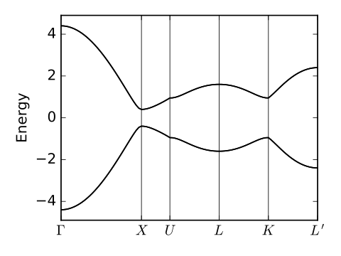
18. fkm.py
#!/usr/bin/env python
from __future__ import print_function # python3 style print
# Three-dimensional Fu-Kane-Mele model
# Fu, Kane and Mele, PRL 98, 106803 (2007)
from pythtb import * # import TB model class
import matplotlib.pyplot as plt
# set model parameters
t=1.0 # spin-independent first-neighbor hop
dt=0.4 # modification to t for (111) bond
soc=0.125 # spin-dependent second-neighbor hop
def set_model(t,dt,soc):
# set up Fu-Kane-Mele model
lat=[[.0,.5,.5],[.5,.0,.5],[.5,.5,.0]]
orb=[[0.,0.,0.],[.25,.25,.25]]
model=tb_model(3,3,lat,orb,nspin=2)
# spin-independent first-neighbor hops
for lvec in ([0,0,0],[-1,0,0],[0,-1,0],[0,0,-1]):
model.set_hop(t,0,1,lvec)
model.set_hop(dt,0,1,[0,0,0],mode="add")
# spin-dependent second-neighbor hops
lvec_list=([1,0,0],[0,1,0],[0,0,1],[-1,1,0],[0,-1,1],[1,0,-1])
dir_list=([0,1,-1],[-1,0,1],[1,-1,0],[1,1,0],[0,1,1],[1,0,1])
for j in range(6):
spin=np.array([0.]+dir_list[j])
model.set_hop( 1.j*soc*spin,0,0,lvec_list[j])
model.set_hop(-1.j*soc*spin,1,1,lvec_list[j])
return model
my_model=set_model(t,dt,soc)
my_model.display()
# first plot: compute band structure
# ---------------------------------
# construct path in k-space and solve model
path=[[0.,0.,0.],[0.,.5,.5],[0.25,.625,.625],
[.5,.5,.5],[.75,.375,.375],[.5,0.,0.]]
label=(r'$\Gamma$',r'$X$',r'$U$',r'$L$',r'$K$',r'$L^\prime$')
(k_vec,k_dist,k_node)=my_model.k_path(path,101)
evals=my_model.solve_all(k_vec)
# band structure plot
fig, ax = plt.subplots(1,1,figsize=(4.,3.))
ax.set_xlim([0,k_node[-1]])
ax.set_xticks(k_node)
ax.set_xticklabels(label)
for n in range(len(k_node)):
ax.axvline(x=k_node[n],linewidth=0.5, color='k')
ax.set_ylabel("Energy")
ax.set_ylim(-4.9,4.9)
for n in range(4):
ax.plot(k_dist,evals[n],color='k')
fig.tight_layout()
fig.savefig("fkm_bsr.pdf")
# second plot: compute Wannier flow
# ---------------------------------
# initialize plot
fig, ax = plt.subplots(1,2,figsize=(5.4,2.6),sharey=True)
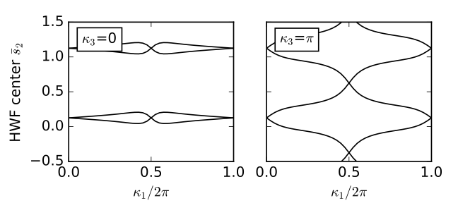
# Obtain eigenvectors on 2D grid on slices at fixed kappa_3
# Note physical (kappa_1,kappa_2,kappa_3) have python indices (0,1,2)
kappa2_values=[0.,0.5]
labs=[r'$\kappa_3$=0',r'$\kappa_3$=$\pi$']
nk=41
dk=1./float(nk-1)
wf=wf_array(my_model,[nk,nk])
#loop over slices
for j in range(2):
for k0 in range(nk):
for k1 in range(nk):
kvec=[k0*dk,k1*dk,kappa2_values[j]]
(eval,evec)=my_model.solve_one(kvec,eig_vectors=True)
wf[k0,k1]=evec
wf.impose_pbc(mesh_dir=0,k_dir=0)
wf.impose_pbc(mesh_dir=1,k_dir=1)
hwfc=wf.berry_phase([0,1],dir=1,contin=True,berry_evals=True)/(2.*np.pi)
ax[j].set_xlim([0.,1.])
ax[j].set_xticks([0.,0.5,1.])
ax[j].set_xlabel(r"$\kappa_1/2\pi$")
ax[j].set_ylim(-0.5,1.5)
for n in range(2):
for shift in [-1.,0.,1.]:
ax[j].plot(np.linspace(0.,1.,nk),hwfc[:,n]+shift,color='k')
ax[j].text(0.08,1.20,labs[j],size=12.,bbox=dict(facecolor='w',edgecolor='k'))
ax[0].set_ylabel(r"HWF center $\bar{s}_2$")
fig.tight_layout()
plt.subplots_adjust(left=0.15,wspace=0.2)
fig.savefig("fkm_topo.pdf")
Printed output
---------------------------------------
report of tight-binding model
---------------------------------------
k-space dimension           = 3
r-space dimension           = 3
number of spin components   = 2
periodic directions         = [0, 1, 2]
number of orbitals          = 2
number of electronic states = 4
lattice vectors:
 #  0  ===>  [     0.0 ,     0.5 ,     0.5 ]
 #  1  ===>  [     0.5 ,     0.0 ,     0.5 ]
 #  2  ===>  [     0.5 ,     0.5 ,     0.0 ]
positions of orbitals:
 #  0  ===>  [     0.0 ,     0.0 ,     0.0 ]
 #  1  ===>  [    0.25 ,    0.25 ,    0.25 ]
site energies:
 #  0  ===>   [[ 0.+0.j  0.+0.j]  [ 0.+0.j  0.+0.j]]
 #  1  ===>   [[ 0.+0.j  0.+0.j]  [ 0.+0.j  0.+0.j]]
hoppings:
<  0 | H |  1 + [  0 ,  0 ,  0 ] >     ===>  [[ 1.4+0.j  0.0+0.j]  [ 0.0+0.j  1.4+0.j]]
<  0 | H |  1 + [ -1 ,  0 ,  0 ] >     ===>  [[ 1.+0.j  0.+0.j]  [ 0.+0.j  1.+0.j]]
<  0 | H |  1 + [  0 , -1 ,  0 ] >     ===>  [[ 1.+0.j  0.+0.j]  [ 0.+0.j  1.+0.j]]
<  0 | H |  1 + [  0 ,  0 , -1 ] >     ===>  [[ 1.+0.j  0.+0.j]  [ 0.+0.j  1.+0.j]]
<  0 | H |  0 + [  1 ,  0 ,  0 ] >     ===>  [[ 0.000-0.125j  0.125+0.j   ]  [-0.125+0.j     0.000+0.125j]]
<  1 | H |  1 + [  1 ,  0 ,  0 ] >     ===>  [[ 0.000+0.125j -0.125+0.j   ]  [ 0.125+0.j     0.000-0.125j]]
<  0 | H |  0 + [  0 ,  1 ,  0 ] >     ===>  [[ 0.+0.125j  0.-0.125j]  [ 0.-0.125j  0.-0.125j]]
<  1 | H |  1 + [  0 ,  1 ,  0 ] >     ===>  [[ 0.-0.125j  0.+0.125j]  [ 0.+0.125j  0.+0.125j]]
<  0 | H |  0 + [  0 ,  0 ,  1 ] >     ===>  [[ 0.000+0.j    -0.125+0.125j]  [ 0.125+0.125j  0.000+0.j   ]]
<  1 | H |  1 + [  0 ,  0 ,  1 ] >     ===>  [[ 0.000+0.j     0.125-0.125j]  [-0.125-0.125j  0.000+0.j   ]]
<  0 | H |  0 + [ -1 ,  1 ,  0 ] >     ===>  [[ 0.000+0.j     0.125+0.125j]  [-0.125+0.125j  0.000+0.j   ]]
<  1 | H |  1 + [ -1 ,  1 ,  0 ] >     ===>  [[ 0.000+0.j    -0.125-0.125j]  [ 0.125-0.125j  0.000+0.j   ]]
<  0 | H |  0 + [  0 , -1 ,  1 ] >     ===>  [[ 0.000+0.125j  0.125+0.j   ]  [-0.125+0.j     0.000-0.125j]]
<  1 | H |  1 + [  0 , -1 ,  1 ] >     ===>  [[ 0.000-0.125j -0.125+0.j   ]  [ 0.125+0.j     0.000+0.125j]]
<  0 | H |  0 + [  1 ,  0 , -1 ] >     ===>  [[ 0.+0.125j  0.+0.125j]  [ 0.+0.125j  0.-0.125j]]
<  1 | H |  1 + [  1 ,  0 , -1 ] >     ===>  [[ 0.-0.125j  0.-0.125j]  [ 0.-0.125j  0.+0.125j]]
hopping distances:
|  pos(  0 )  - pos(  1 + [  0 ,  0 ,  0 ] ) |  =     0.433
|  pos(  0 )  - pos(  1 + [ -1 ,  0 ,  0 ] ) |  =     0.433
|  pos(  0 )  - pos(  1 + [  0 , -1 ,  0 ] ) |  =     0.433
|  pos(  0 )  - pos(  1 + [  0 ,  0 , -1 ] ) |  =     0.433
|  pos(  0 )  - pos(  0 + [  1 ,  0 ,  0 ] ) |  =    0.7071
|  pos(  1 )  - pos(  1 + [  1 ,  0 ,  0 ] ) |  =    0.7071
|  pos(  0 )  - pos(  0 + [  0 ,  1 ,  0 ] ) |  =    0.7071
|  pos(  1 )  - pos(  1 + [  0 ,  1 ,  0 ] ) |  =    0.7071
|  pos(  0 )  - pos(  0 + [  0 ,  0 ,  1 ] ) |  =    0.7071
|  pos(  1 )  - pos(  1 + [  0 ,  0 ,  1 ] ) |  =    0.7071
|  pos(  0 )  - pos(  0 + [ -1 ,  1 ,  0 ] ) |  =    0.7071
|  pos(  1 )  - pos(  1 + [ -1 ,  1 ,  0 ] ) |  =    0.7071
|  pos(  0 )  - pos(  0 + [  0 , -1 ,  1 ] ) |  =    0.7071
|  pos(  1 )  - pos(  1 + [  0 , -1 ,  1 ] ) |  =    0.7071
|  pos(  0 )  - pos(  0 + [  1 ,  0 , -1 ] ) |  =    0.7071
|  pos(  1 )  - pos(  1 + [  1 ,  0 , -1 ] ) |  =    0.7071

----- k_path report begin ----------
real-space lattice vectors
 [[ 0.   0.5  0.5]
 [ 0.5  0.   0.5]
 [ 0.5  0.5  0. ]]
k-space metric tensor
 [[ 3. -1. -1.]
 [-1.  3. -1.]
 [-1. -1.  3.]]
internal coordinates of nodes
 [[ 0.     0.     0.   ]
 [ 0.     0.5    0.5  ]
 [ 0.25   0.625  0.625]
 [ 0.5    0.5    0.5  ]
 [ 0.75   0.375  0.375]
 [ 0.5    0.     0.   ]]
reciprocal-space lattice vectors
 [[-1.  1.  1.]
 [ 1. -1.  1.]
 [ 1.  1. -1.]]
cartesian coordinates of nodes
 [[ 0.    0.    0.  ]
 [ 1.    0.    0.  ]
 [ 1.    0.25  0.25]
 [ 0.5   0.5   0.5 ]
 [ 0.    0.75  0.75]
 [-0.5   0.5   0.5 ]]
list of segments:
  length =     1.0  from  [ 0.  0.  0.]  to  [ 0.   0.5  0.5]
  length = 0.35355  from  [ 0.   0.5  0.5]  to  [ 0.25   0.625  0.625]
  length = 0.61237  from  [ 0.25   0.625  0.625]  to  [ 0.5  0.5  0.5]
  length = 0.61237  from  [ 0.5  0.5  0.5]  to  [ 0.75   0.375  0.375]
  length = 0.61237  from  [ 0.75   0.375  0.375]  to  [ 0.5  0.   0. ]
node distance list: [ 0.       1.       1.35355  1.96593  2.5783   3.19067]
node index list:    [  0  31  42  62  81 100]
----- k_path report end ------------
fkm_bsr.pdf
fkm_topo.pdf